
Introduction
Have you ever wondered how a Large Language Model (LLM) like ChatGPT actually reads and understands text? The answer begins with something called a tokenizer.
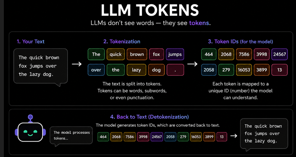
A tokenizer is the very first step in the language processing pipeline. Before an AI model can understand a sentence, answer a question, or generate text, it must first break the input into smaller pieces called tokens. These tokens are the units the model uses to process language internally.
What is a Token and Tiktoken?
A token can be many different things. Sometimes it is a complete word, such as “football.” In other cases, it can be only a part of a word. For example, the word “extraordinary” might be split into smaller pieces like “extra”, “ordin”, and “ary.” Tokens can also include punctuation marks, spaces, symbols, emojis, or even URLs.
After the text is divided into tokens, each token is assigned a unique numeric ID from the tokenizer’s vocabulary. In simple terms, tokenization is the bridge between human language and machine understanding, making it one of the most important concepts in modern AI and Large Language Models.
So, we are using tiktoken, an open-source library developed by OpenAI, to understand how text is converted into tokens. It uses the same tokenization method as OpenAI’s models, allowing us to see exactly how words, punctuation, and symbols are split before being processed by an LLM. This makes it a useful tool for learning how tokenization works and for estimating token usage in real-world applications. tiktoken was introduced to provide a reliable and consistent way for developers to work with the tokenization schemes used by models such as GPT-3.5 and GPT-4, helping bridge the gap between raw text and the numerical representations that LLMs
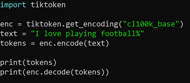
The code above demonstrates how the cl100k_base tokenizer converts the text “I love playing football%” into a sequence of token IDs that a Large Language Model can understand and process. Each word, symbol, or character is broken into tokens, and every token is mapped to a unique numeric value from the tokenizer’s vocabulary.
The `tokens` list represents these numeric IDs, while enc.decode(tokens) performs the reverse operation by converting the token IDs back into the original text. In simple terms, this example shows the complete flow of how LLMs handle text internally: Text → Tokens → Token IDs → Text.

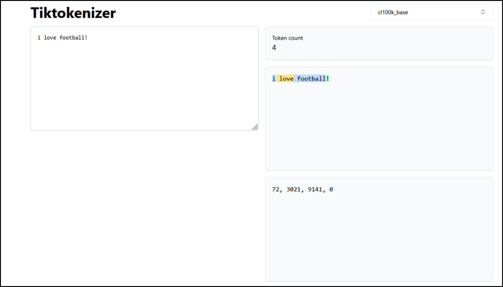
For example, a sentence like “I love playing football!” may be transformed into a sequence of token IDs such as [40, 3021, 5737, 9141, 4]. While humans see readable text, the model only works with these numerical representations internally.
Each token ID corresponds to a specific word, subword, or symbol stored in the tokenizer’s vocabulary. Since transformer models can only process numerical data, these token IDs are converted into vectors of numbers called embeddings. The model performs all of its computations on these vectors and produces another vector as output. During text generation, this output is used to predict the most likely next token, which is then converted back into human-readable text by the tokenizer.

For example, in this tokenizer, the exclamation mark “!” is assigned the token ID 0 based on its position within the tokenizer’s vocabulary. Every word, symbol, or character is mapped to a unique numeric ID that the model uses internally during processing.
The enc.decode(tokens) function performs the reverse operation by converting those token IDs back into human-readable text. This demonstrates the complete workflow used inside Large Language Models: Text → Tokens → Token IDs → Text. If you want to experiment with tokenization yourself, you can also use the tokenizer visualizer available at https://tiktokenizer.vercel.app/?model=cl100k_base, which allows you to see how text is split into tokens and mapped to IDs in real time.
Modern Tokenization and Workflow in LLMs
Modern Large Language Models (LLMs) cannot process raw text directly because neural networks only work with numerical data. Tokenizers solve this problem by breaking text into smaller units called tokens and assigning each token a unique numeric ID.
Modern tokenizers commonly use subword-based techniques such as Byte Pair Encoding (BPE), WordPiece, and SentencePiece. These methods allow models to efficiently handle rare words, multiple languages, misspellings, and previously unseen terms without requiring an extremely large vocabulary. As a result, the model can generalize more effectively while keeping the vocabulary size manageable.
The overall text processing pipeline inside an LLM can be simplified as:
Raw Text → Tokenization → Token IDs → Embedding Vectors → Neural Network → Output Token IDs → Text
Tokens to Embeddings
After text is converted into tokens, the LLM still cannot work with just token IDs because numbers like 40, 3021, 5737, 9141 don’t carry meaning by themselves. To understand language, the model needs a way to represent each token in a format that captures semantic relationships, meaning, context, similarity, and grammar. This is achieved through embeddings.
To make tokens meaningful, the model converts each token ID into an embedding vector. An embedding is a continuous high-dimensional vector representation of a token that helps the model capture semantic relationships, patterns, and similarities between words.
Instead of representing a token as a single number, embeddings transform it into a dense vector of floating-point values. These vectors allow the model to learn relationships between words, grammar, and language structure during training.
For example, words with similar meanings often end up with embedding vectors that are mathematically close to each other in vector space. This is one of the key reasons embeddings are fundamental to how Large Language Models understand and generate human language.
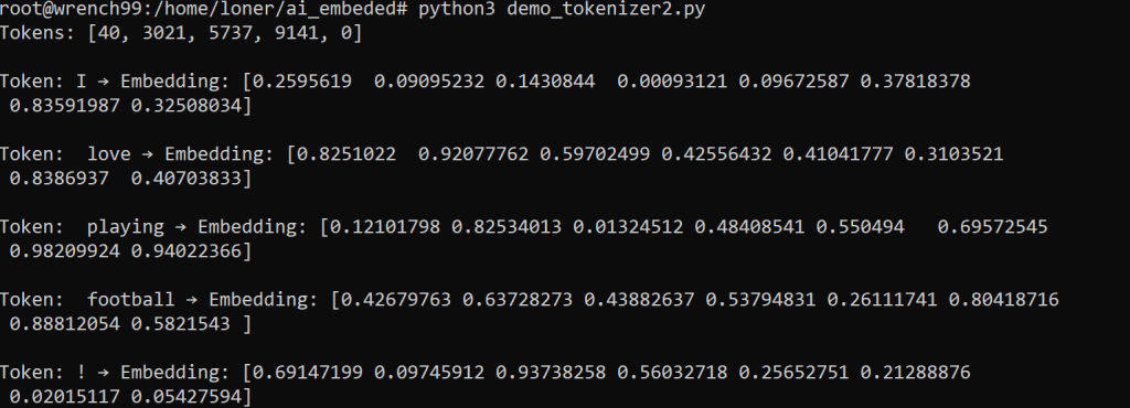
The code first tokenizes the input text using the cl100k_base tokenizer, converting each word and symbol into numeric token IDs. Since neural networks cannot process token IDs directly, the code then simulates an embedding layer by creating a random embedding table containing 100,000 rows one for each possible token in the vocabulary and 8 columns representing the embedding dimensions. Each token ID is used to retrieve its corresponding embedding vector, allowing the model to represent tokens as meaningful numerical features instead of simple integer values.

Each token ID is then used as an index to retrieve its corresponding embedding vector from the embedding table. Finally, the script prints every token alongside its embedding vector, demonstrating how raw text is transformed into dense numerical representations that a neural network can process.
| Model | Embedding Dimension |
| GPT-2 Small | 768 |
| GPT-3 175B | 12,288 |
| GPT-4 (estimated) | 25,600+ |
These embedding vectors help the model measure semantic similarity between words. For example, words related to sports such as football and cricket may have embedding vectors that are closer together in vector space, while unrelated words like football and potato are likely to be farther apart.
Once tokens are converted into embeddings, the model can perform mathematical operations such as matrix multiplication, attention mechanisms, and gradient updates. This allows the neural network to learn patterns, relationships, grammar, and contextual information from language data.
In simple terms, embeddings transform symbolic text into dense numerical representations that Large Language Models can use to understand and generate human language.
Step 3 – Embeddings → Neural Network (Attention + Prediction)
Once each token is converted into an embedding vector, the LLM processes these vectors through its neural network layers to understand context and predict the next token. The most important mechanism inside modern LLMs is Self-Attention. Attention allows the model to decide which words should influence each other. For example, in the sentence “He kicked the ball because it was flat”, the model learns that “it” refers to the ball, not “he”.
Understanding Self-Attention in LLMs
Self-attention is the core mechanism that enables a Large Language Model (LLM) to understand relationships between words in a sentence. Instead of processing each word independently, self-attention allows every token to “look at” other tokens and determine which ones are most important for understanding the overall meaning. For example, in the sentence “I love playing football!”, the word “I” is closely related to “love”, while “playing” is strongly connected to “football.” By calculating these relationships mathematically, self-attention creates context-aware representations that help the model understand words based on their surrounding context rather than in isolation.
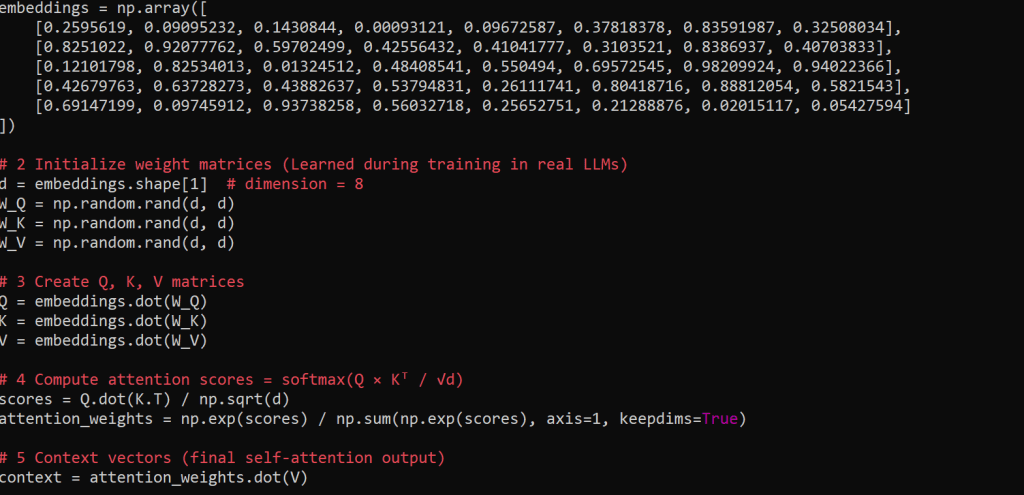
In the Python script above, the token embeddings are passed through a simplified Transformer self-attention mechanism. First, the embedding vectors for each token (I, love, playing, football, !) are loaded. Then, three learned weight matrices W_Q (Query), W_K (Key), and W_V (Value) are used to generate the Query, Key, and Value vectors. These vectors help the model determine what each token is searching for (Query), what information it contains (Key), and what information it contributes to other tokens (Value). The script computes attention scores by comparing the Query vectors with the Key vectors, then applies the softmax function to normalize these scores into attention weights.
What is Softmax?
Before selecting the next token, the model produces a set of raw scores called logits, where each score represents how likely a token is to be chosen. These logits are passed through a function called Softmax, which converts them into probabilities. Softmax scales the values so that each probability falls between 0 and 1, and all probabilities add up to 100%. This is important because the raw logits themselves are not easy to interpret. By converting them into probabilities, the model can compare all possible tokens and select the most likely next token in a mathematically meaningful way.

Finally, the attention weights are multiplied with the Value vectors to generate context vectors, which represent each token with sentence-level contextual meaning.
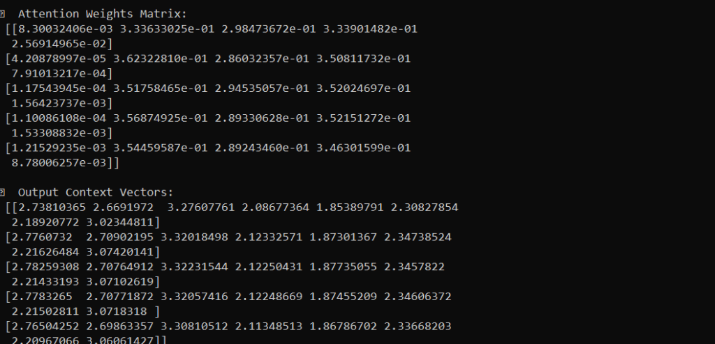
These context vectors are then passed to the next Transformer layer, enabling the model to learn language patterns and predict the next token in real LLMs.
Step 4 – Feed-Forward Layer (Simple Explanation)
After the attention mechanism combines information from all the words in a sentence, each token is passed through another component called the feed-forward layer. This is a small neural network applied independently to every token. The layer first expands the token into a larger representation to learn more complex patterns and then compresses it back to its original size.
In simple terms, attention allows words to communicate with each other, while the feed-forward layer helps each word refine and improve its own understanding based on the information gathered from the sentence. This process helps the model build a deeper understanding of context before passing the data to the next Transformer layer.
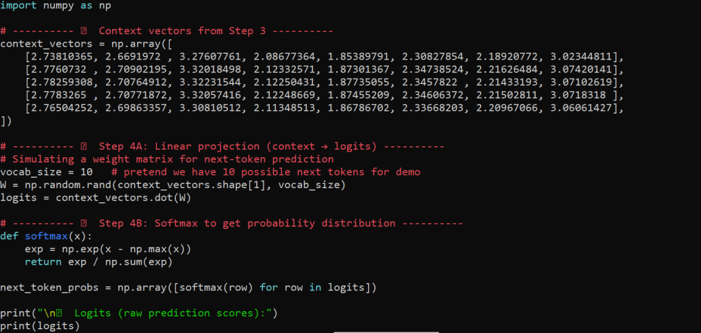
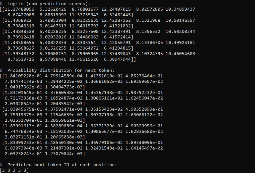
In this step, the model uses the context vectors generated by self-attention to predict the next token. First, these context vectors are multiplied by a learned weight matrix W, which transforms the contextual information into logits raw scores representing how likely each token in the vocabulary is to appear next. The model then applies the softmax function, which converts these raw scores into probabilities where all values are positive and add up to 1. Finally, the model selects the token with the highest probability using the argmax operation. In simple words: context → scores → probabilities → predicted next token.
Step 5 – Decode Predicted Token to Text (Explanation)
After the model predicts the next token IDs in Step 4, the final step is to convert those numeric IDs back into human-readable text. In this example, the model predicted the token ID 3 for every position in the sequence. The tokenizer’s decode function is then used to map each token ID back to its corresponding word, symbol, or subword stored in the vocabulary.
For example, if token ID 3 corresponds to the symbol “$”, the decoded output becomes:
[‘$’, ‘$’, ‘$’, ‘$’, ‘$’]
which produces the final predicted sentence:
$$$$$ This step demonstrates how Large Language Models transform internal numerical predictions back into readable text that humans can understand.

In this simple demo, the model predicts the symbol “$” repeatedly because the weights and embeddings are randomly generated and not actually trained on real language data. Since the model has not learned grammar, sentence structure, or word relationships, its predictions are essentially random mathematical outputs. In this case, the token ID with the highest probability happened to map to the symbol “$” in the tokenizer’s vocabulary. Real Large Language Models are trained on massive datasets and learn meaningful patterns between words, allowing them to generate sensible predictions. However, in this simplified example, the goal is only to demonstrate the workflow of how token IDs are predicted and then decoded back into text, not to generate meaningful language.
Byte Pair Encoding (BPE)
Byte Pair Encoding is a frequency-based subword tokenization algorithm. It was originally a compression algorithm, but it was adapted for NLP because it solves a key problem: how to reduce vocabulary size while still being able to represent unknown words. If we tokenize by full words, the vocabulary becomes extremely large and cannot handle new words. If we tokenize by characters, sequences become too long and inefficient.
BPE finds a middle ground by starting with individual characters and repeatedly merging the most frequent adjacent character pairs. Over time, common patterns like “th”, “ing”, “low”, etc., become single tokens.
The training process works like this:
- Start with a corpus of text.
- Split every word into characters.
- Count all adjacent symbol pairs.
- Merge the most frequent pair into a new token.
- Repeat this process many times.
- Store all merge operations in order.
Define and Prepare the Corpus (BPE)
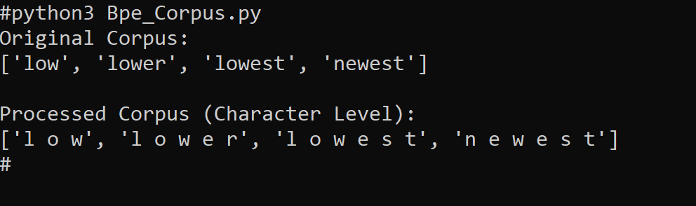
In Byte Pair Encoding (BPE), the first step is to define and prepare the corpus, which is simply a collection of words or sentences that the algorithm will learn from. Before BPE can start learning patterns, each word in the corpus must be broken down into individual characters, and those characters must be separated by spaces. For example, the word “low” becomes “l o w.”
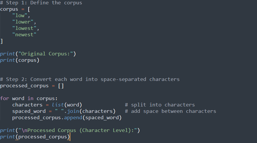
This is important because BPE starts from the smallest units, which are characters, and then gradually merges the most frequent character pairs to form bigger pieces. By separating characters clearly at the beginning, we allow the algorithm to see and count adjacent pairs correctly, which is how it learns to build meaningful subword tokens step by step.
Counting Adjacent Pairs
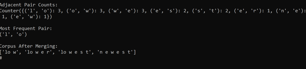
After converting every word into space-separated characters, the next step in Byte Pair Encoding (BPE) is to count all adjacent character pairs. This means we look at each word and take two neighboring symbols at a time. For example, in “l o w”, the pairs are (l, o) and (o, w). We do this for every word in the processed corpus and count how many times each pair appears.
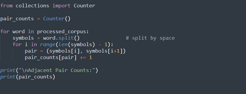
The main goal of this step is to find the most frequent pair, because BPE always merges the pair that appears the most. This counting step is important since BPE is completely based on frequency; the most common pair will become the next new token.

Merge the Most Frequent Pair
After counting all adjacent pairs, we now find the pair that appears the most and merge that pair everywhere in the corpus. This means we replace the two separate symbols with one combined token.
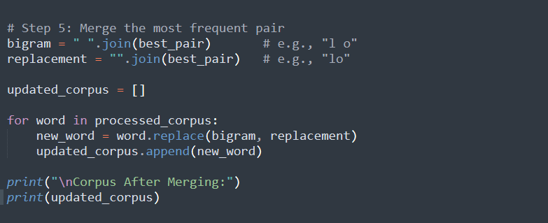
For example, if (l, o) is the most frequent pair, we replace “l o” with “lo” in all words. After merging, the corpus changes, and we can repeat the process again.
Repeat the Process (Loop Until Done)
After merging the most frequent pair once, BPE does not stop. The next step is to repeat the same process again and again. Every time we merge a pair, the corpus changes. Because the corpus changes, the adjacent pairs also change. So we must count pairs again, find the new most frequent pair, and merge it again. This loop continues for a fixed number of merges or until no more pairs are left. Step by step, small characters become bigger subword tokens like “lo”, then “low”, then maybe “lowest”. This repeating process is what slowly builds the vocabulary.
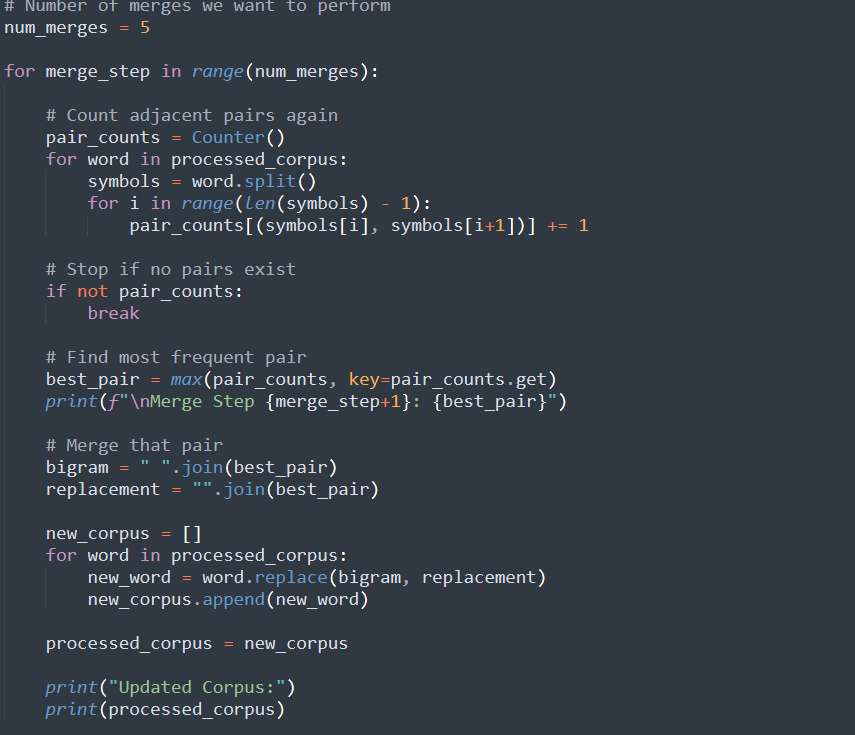
The output shows how BPE is slowly building bigger tokens step by step. By step 5, the pair (‘lowe’, ‘r’) was the most frequent, so it merged them into the single token “lower”. That is why “lower” now appears as one complete token in the corpus. Other words like “lowest” and “newest” are still partially split (for example, “lowe st”), because those pairs were not the most frequent yet.
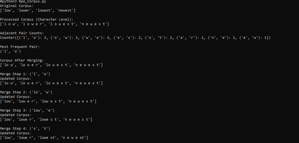
This shows that BPE merges common patterns first and leaves less frequent patterns split until later steps.
Conclusion
In this blog, we explored the fundamental concepts behind how Large Language Models (LLMs) process and generate text. We started with tokenization and examined how text is broken into tokens, including a practical walkthrough of Byte Pair Encoding (BPE) to understand how subword tokens are created. We then saw how tokens are converted into embedding vectors, allowing the model to represent language as numerical data. Through self-attention and feed-forward layers, the Transformer architecture learns context and relationships between tokens to make predictions. Finally, the model selects the most likely next token and converts it back into human-readable text. Together, these concepts form the foundation of modern Transformer-based LLMs and provide a deeper understanding of how models generate meaningful language.